|
Getting your Trinity Audio player ready...
|
In a previous Montaka article on the differences between investing and gambling, the point was made that “when determining the value of any asset it is important to think probabilistically – that is, acknowledging that there are many possible outcomes that can eventuate in the future”. A thorough analysis of a business involves a consideration of the many future scenarios that may occur, as well as a calculation of the intrinsic value of the business under each scenario. But is there a way to distill this spectrum of possible values for a business into a single number?
Statistics courses teach that this can be achieved by calculating an expected value, that is, a predicted value that’s calculated from the sum of all possible values after each are multiplied by the probability of that value’s occurrence. The mathematical formula for expected value appears below:
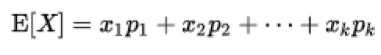
Where some random variable X can take the value X1, with probability p1, and so forth up to value Xk with probability pk.
It is worth exploring an example to see where and how an expected value might be used. Imagine a hypothetical business that produces military uniforms for the U.S. government. This business has a contract to produce uniforms for its sole customer, the U.S. Department of Defense, and has no other lines of business.
An investor trying to value this business must acknowledge the extreme customer concentration and the two key scenarios that will impact the intrinsic value of the business: (i) the business maintains the government contract, and in this scenario the firm will be valued based on the cash flows it is estimated to produce over its lifetime; or (ii) the business loses the government contract and is worth zero (although in reality there is likely to be some residual value if assets such as land or equipment can be sold off).
The table below displays the abovementioned outcomes and attaches a probability to these two binary events.
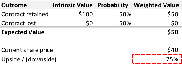
If one were to assume a 50:50 chance of either event occurring, with the business worth $100 if it keeps the government contract and $0 if it loses the contract, then the expected value of the business is $50. A value investor scouring the universe for cheap stocks might get excited when they see that the stock price of this company is $40, or 25% upside from the $50 expected value. Surely this is a bet one would take time and time again?
Despite the large upside, the attractiveness of this investment opportunity is superficial at best. The investment is a classic example of the average telling lies and reminds us of the statistician who put his head in an oven and his feet in a freezer, proclaiming, “On average, I feel fine”. What the expected value analysis ignores is the extreme distribution of outcomes; although the expected value and “business as usual” scenarios appear very favorable from a returns perspective, the prospect of losing the government contract presents unpalatable downside risk. This is an unattractive bet in isolation and in fact little can be done to diversify away this risk.
In theory, if you were able to find many of the exact same situations and place multiple bets on that same situation, your investment return should converge towards 25% as the number of investments increases. However, in reality it is impossible to construct a portfolio of many of these exact same situations, given that each investment has its own nuanced risk/reward characteristics and the probabilities of these situations will most likely be uncorrelated.
One of the pithiest condemnations of the expected value as a tool for decision making was by Daniel Bernoulli in the Commentaries of the Imperial Academy of Science of Saint Petersburg. The so called St. Petersburg paradox involves a casino game of chance where a player’s initial stake of $2 is doubled every time the toss of fair coin lands on heads. When the coin first lands on tails, the game is stopped and the player wins the sum that is accumulated.
For example, if the coin lands on heads in the first toss, the wagered sum of $2 doubles to $4. If tails appear on the second toss, then the game ends and player walks away with $4. If instead heads appear on the second toss, then the prize doubles to $8, and so on. The mathematical representation of this is shown below, and yields an infinite expected value.
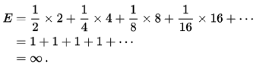
How much would you pay for each play of this casino game? A paradox arises because the infinite expected value suggests that the winnable prize is infinite, yet it is likely that someone would pay only a small price to play this game in reality.
The expected value concept is flawed and oversimplifies the complexity of future events that can occur. It may be the case that false conclusions are drawn about the risk/reward trade-off for an investment as a result of using this concept. As such, the Montaka team prefers to think about possible future outcomes using a Bayesian framework, which was discussed in a recent Montaka post.
![]() George Hadjia is a Research Analyst with Montgomery Global Investment Management. To learn more about Montaka, please call +612 7202 0100.
George Hadjia is a Research Analyst with Montgomery Global Investment Management. To learn more about Montaka, please call +612 7202 0100.