|
Getting your Trinity Audio player ready...
|
In my previous post I delved into some of the technical terms and mathematical relationships that are necessary to understand the performance of long/short funds. Since then we have had some great feedback from a range of readers which has prompted me to expand on the topic – with a few more equations and numbers. This memo will illustrate the power of an additional driver available to long/short funds to enhance performance: variable net exposure.
The previous chapter
Taking the mathematical derivation as read and understood, we know that the return of a long/short fund can be represented by the following equation:
rF = gL* αL+ gS* αS + rM* (gL– gS);
where:
rF is the return of the long/short fund;
gLis the long (gross) exposure of the fund;
gSis the short (gross) exposure of the fund;
αLis the long alpha, or outperformance of the long portfolio over the market;
αSis the short alpha, or outperformance of the short portfolio over the inverse of the market; and,
rMis the return of the market.
We also broke this equation into three components of long/short fund performance as follows:
- Outperformance of the long portfolio, scaled by the gross long exposure: (gL* αL)
- Outperformance of the short portfolio, scaled by the short gross exposure: (gS* αS)
- Market return scaled by the “net market exposure” which is the difference between long and short gross exposures: rM* (gL– gS)
To this point in our discussion we have assumed over any time frame that the g’s (and the α’s too) are fixed parameters. However, the long/short fund manager may vary the long and short exposures and therefore the resulting net exposure (gL– gS) of the fund to the market return. Clearly as the g’s vary independently the outperformance components (1 and 2, above) of the fund’s return will change. However, for the purpose of this article we will keep these return components fixed[1]. Our focus will be on the impact on the fund’s performance from varying the net market exposure.
Variable net as a source of alpha
Let’s go back to the original numerical example from last time where we assume our fund is 90% gross long, 50% gross short, that we can generate 5% of alpha on the long side, 3% of alpha on the short side, and the market return is 8%. We can also assume that these are average annual returns so that the average annual return of the long/short fund is:
rF = (90% * 5%) + (50% * 3%) + 8% * (90% – 50%) = 9.2%
In a nutshell this example demonstrated that even with the drag of being less than fully exposed to the market (net exposure is just 40%), a long/short fund can outperform the market even when the market produces solid positive performance on average. But the long/short fund can do more still.
To extend our example let’s assume that the market (simply) averaged 8% p.a. for 10 years, but that performance in any given year is as follows:
![]()
We are going to continue to assume the fund generates scaled long outperformance of 4.5% p.a. (component 1) and scaled short outperformance of 1.5% p.a. (component 2). Therefore, combined outperformance components remain fixed at 6% p.a.*
Importantly, however, we are now going to assume that the manager can and does vary the net market exposure of the fund. Specifically, when stocks are expensive and subsequently underperform their 10-year average return in any year, the manager will only have 20% of the fund exposed to the market. When stocks are cheap and subsequently outperform their 10-year average return in any year, the manager will have 60% of the fund exposed to the market. This is shown below:

We can now calculate the market-related return component of the long/short fund’s performance in each year by multiplying the market return by the net market exposure for that period i.e. rM* (gL– gS) or component 3. The result is shown here:

We can see that the ability to vary the net exposure of the fund has resulted in 5.6 percentage points per annum of market-related return, which compares to 3.2 percentage points per annum when the net exposure was fixed at 40% i.e. 8% * (90% – 50%) = 3.2%. This increases the overall annual average return of the long/short fund to 11.6%.
In other words, the ability to vary the net exposure is another source of alpha and a fourth component of returns that we had not explicitly broken out previously. In addition to the 6% p.a. contribution from the outperformance of long and short books, and the 3.2% contribution from the average net market exposure of 40%, the variable net exposure has added another 2.4% to the performance of the long/short fund in this example.
Montaka’s variable net
Historically the net market exposure of Montaka has varied as a result of the bottom-up availability of good long and short opportunities, as well as our top-down view of the risk environment and stock price levels. Andrew Macken explains the latter in more detail in his recent post here.
Montaka’s net market exposure over the last year and a half is shown below. It should be clear that on balance the fund has been relatively less exposed to markets when stock prices and risks have become elevated, and relatively more exposed to markets as both factors have become more favourable (lower equity prices and less chance of negative risks eventuating).
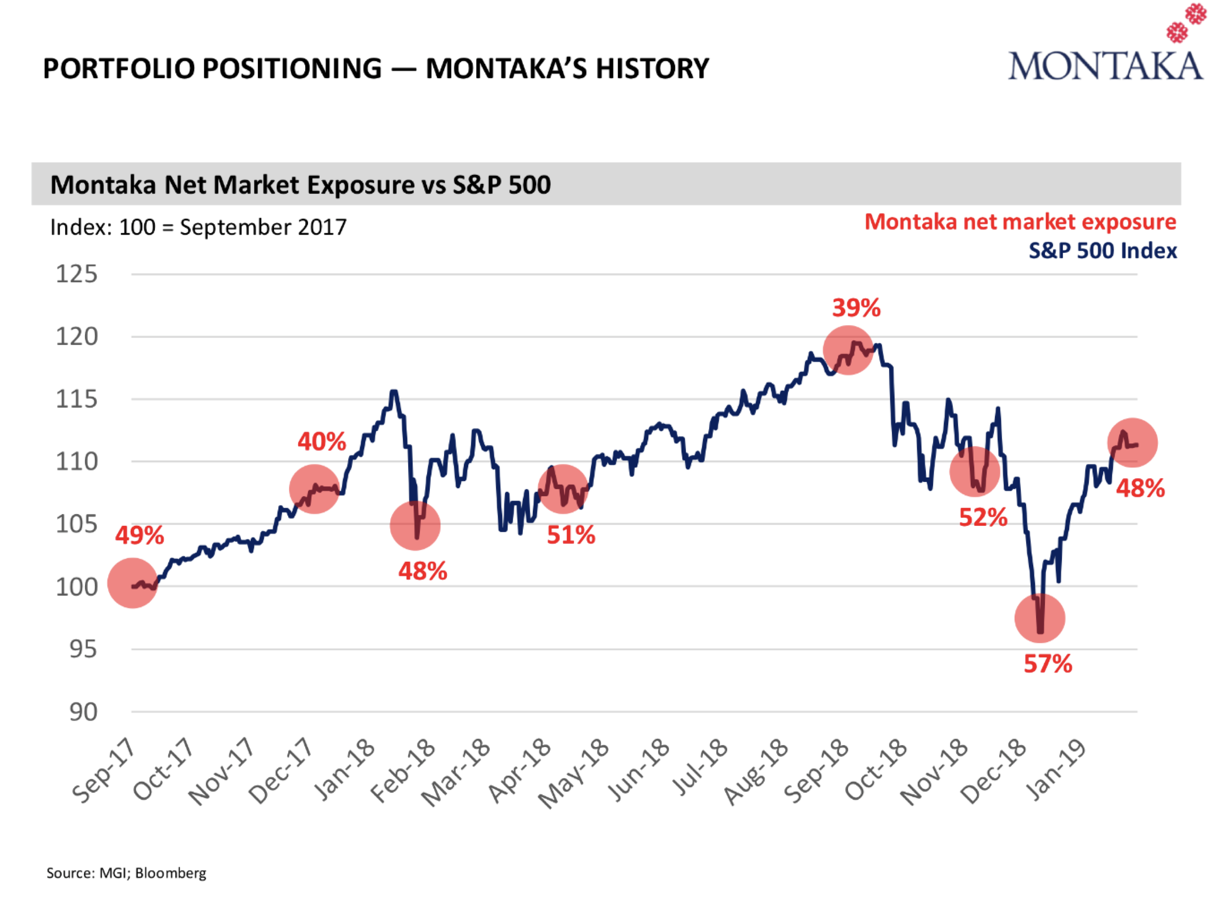
As markets move and risks change, we will continue to use Montaka’s variable net exposure as a key lever to add value for our clients.
[1]In reality, a varying net exposure would necessitate varying gross long and short exposures. For the purpose of the example we have fixed the result of the outperformance components and therefore implicitly assumed that any change in exposures (g’s) is offset by changes in outperformance (α’s). This is not unreasonable, nor does it change the result of the analysis.
![]()
Christopher Demasi is a Portfolio Manager with Montaka Global Investments.
To learn more about Montaka, please call +612 7202 0100.